Visualizing GoogLeNet Classes
Ever wondered what a deep neural network thinks a Dalmatian should look like? Well, wonder no more.
Recently Google published a post describing how they managed to use deep neural networks to generate class visualizations and modify images through the so called “inceptionism” method. They later published the code to modify images via the inceptionism method yourself, however, they didn’t publish code to generate the class visualizations they show in the same post.
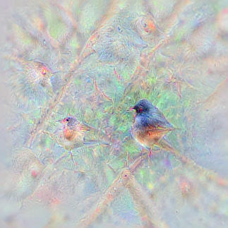
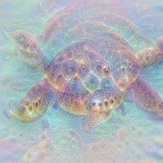
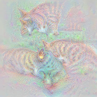
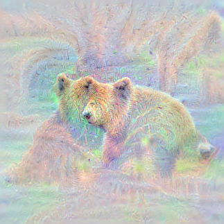
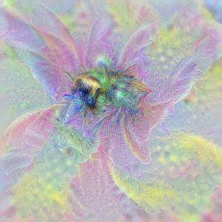
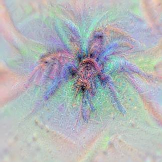
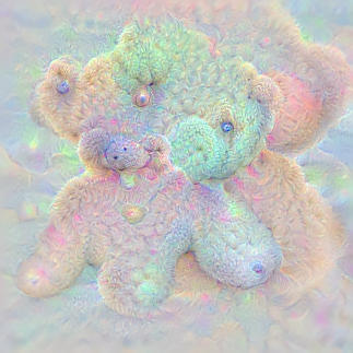
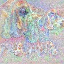
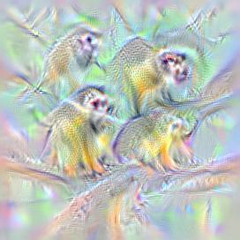
While I never figured out exactly how Google generated their class visualizations, after butchering the deepdream code and this ipython notebook from Kyle McDonald, I managed to coach GoogLeNet into drawing these:
It should be mentioned that all of these images are generated completely from noise, so all information is from the deep neural network, see an example of the gradual generation process below:
In this post I’ll describe a bit more details on how I generated these images from GoogLeNet, but for those eager to try this out yourself, jump over to github where I’ve published ipython notebooks to do this yourself. For more examples of generated images, see some highlights here, or visualization of all 1000 imagenet classes here.
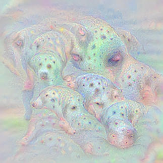
Aside from the fact that our network seems to be drawing with rainbow crayons, it’s remarkable to see how detailed the images are. They’re far from perfect representations of the objects, but they give us valuable insight into what information the network thinks is essential for an object, and what isn’t. For instance, the tabby cats seem to lack faces while the dalmatians are mostly dots. Presumably this doesn’t mean that the network hasn’t learned the rest of the details of these objects, but simply that the rest of the details are not very discriminate characteristics of that class, so they’re ignored when generating the image.
As google also noted in their post, there are often also details that actually aren’t part of the object. For instance, in this visualization of the “Saxophone” class there’s a vague saxophone player holding the instrument:
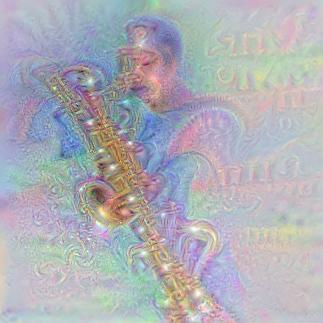
This is presumably because most of the example images used for training had a saxophone player in them, so the network sees them as relevant parts of the object.
In the next part I’ll go a bit into details on how the gradient ascent is done. Note : this is for specially interested, with some knowledge of deep neural networks being necessary.
Generating class visualizations with GoogLeNet
In order to make a deep neural network generate images, we use a simple trick. Instead of using backpropagation to optimize the weights, which we do during training, we keep the weights fixed and instead optimize the input pixels. However, trying to use unconstrained gradient ascent to get a feasible class visualization works poorly, giving us images such as the one below.
The reason for this is that our unconstrained gradient ascent quickly runs into local maximums that are hard to get out of, with high frequency and low frequency information competing and creating noise. To get around this, we can choose to just optimize the low-frequency information first, which will give us the general structure of the image, and then gradually introduce high-frequency details as we continue gradient ascent, in effect “washing out” an image. Doing this in a slow way, we manage to ensure that optimization converges with a feasible image. There are two possible routes for doing this:
- applying gaussian blur to the image after we’ve applied the gradient step, starting with a large sigma and slowly decreasing it as we iterate
- applying gaussian blur to the gradient, starting with a large sigma and slowly decreasing it as we iterate (note that in this case we also have to use L2-regularization of the pixels to gradually decrease irrelevant noise from previous iterations)
I’ve had best results with the former approach, which is the approach I used to generate the images above, but it might be that someone might get better results with blurring the gradient via messing about with the parameters some more.
While this approach works okayish for relatively shallow networks like Alexnet, a problem you’ll quickly run into when doing this with GoogLeNet, is that as you gradually reduce the amount of blurring applied, the image gets saturated with high-frequency noise like this:
The reason for this problem is a bit uncertain, but might have to do with the depth of the network. In the original paper describing the GoogLeNet architecture, the authors mention that since the network is very deep, with 22 layers, they had to add two auxiliary classifiers at earlier points in the network to efficiently propagate gradients from the loss all the way back to the first layers. These classifiers, which were only used during training, ensured proper gradient flow and made sure that early layers were getting trained as well.
In our case, the pixels of the image are even further ahead in the network than first layer, so it might not seem so surprising that we have some problems with gradients and recovering a feasible image. Exactly why this affects high-frequency information more than low-frequency information is a bit hard to understand, but it might have to do with gradients for high-frequency information being more sensitive and unstable, due to larger weights for high-frequency information, as mentioned by Yosinski in the appendix to this paper.
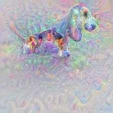
While the auxiliary classifiers in GoogleNet are only used during training, there’s nothing stopping us from using them for generating images. Doing gradient ascent on the first auxiliary classifier, we get this:
while the second auxiliary classifier gives us this:
As can be seen, the first classifier easily manages to generate an image without high-frequency noise , probably because it’s “closer” to the early layers. However, it does not retain the overall structure of the object, and peppers the image with unnecessary details. The reason for the lack of structure is that the deeper a network is, the more structure the network is able to learn. Since the first classifier is so early in the network, it has not yet learned all of the structures deeper layers has. We can similarly see that the second classifier has learned some more structure, but has slightly more problems with high-frequency noise (though not as bad as the final classifier).
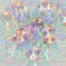
So, is there any way to combine the gradients from these classifiers in order to ensure both structure and high-frequency information is retained? Doing gradient ascent on all three classifiers at the same time unfortunately does not help us much, as we get both poor structure and noisy high-frequency information. Instead, what we can do is to first do gradient ascent from the final classifier, as far as we can before we run into noise, then switch to doing gradient ascent from the second classifier for a while to “fill in” details, then finally switching to doing gradient ascent from the first classifier to get the final fine-grained details.
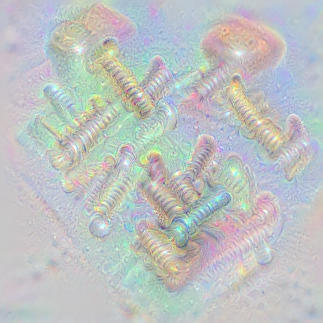
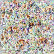
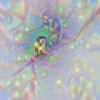
Another trick we used, both to get larger images and better details, was to scale up the image at certain intervals, similar to the “octaves” used in the deepdream code. Since the input image the network optimizes is restricted to 224x224 pixels, we randomly crop a part of the scaled up image to optimize at each step. Altogether, this gives us this result:

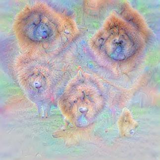
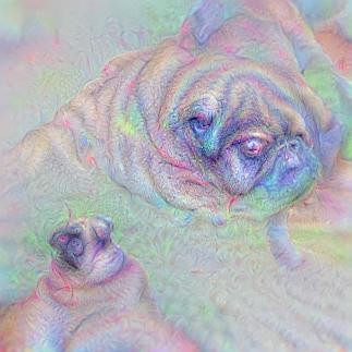
Though this approach gives us nicely detailed images, note that both the scaling and the auxiliary classifiers tend to degrade the overall structure of the image, and particularly larger objects often tend to be “torn apart”, such as this dog gradually turning into multiple dogs.
Since the network actually seems to be capable of creating more coherent objects, it’s possible that we could generate better images with clever priors and proper learning rates, though I didn’t have any luck with it so far. Purely hypothetically, deep networks with better gradient flow might also be able to recover more detailed and structured images. I’ve been curious to see if networks with batch normalization or Parametric ReLUs are better at generating images since they seem to have better gradient flow, so if anyone has a pretrained caffe model with PReLUs or batch normalization, let me know!
Another detail that’s worthy to note is that we did not optimize directly the loss layer, as the softmax denominator makes the gradient ascent put too much weight on reducing other class probabilities. Instead, we optimize the next to last layer, where we can make the gradient ascent focus exclusively on optimizing a likely image from our class.
As a final side note it’s very interesting to compare the images AlexNet and GoogLeNet generate. While the comparison might not be entirely representative, it certainly looks like Googlenet has learned a lot more details and structure than AlexNet.
Now go ahead and try it yourself! If you figure out other tricks or better choices of parameters for the gradient ascent (there almost certainly are), or just create some cool visualizations, let me know via twitter!
A big hat tip to google and their original deepdream code, as well as Kyle McDonald, which had the original idea of gradually reducing sigma of gaussian blurring to “wash out” the image, and kindly shared his code.