Fitting faces
An explanation of clmtrackr
A while ago I put out a semi-finished version of CLMtrackr, which is a javascript library for fitting a facial model to faces in images or video. Fitting a facial model is useful in cases where you need precise positions of facial features, such as for instance emotion detection, face masking and person identification. Though the tracking is pretty processor-intensive, we manage to reach real-time tracking in modern browsers, even though it’s implemented in javascript. If you’re interested in seeing some applications of CLMtrackr, check out the demos of face substitution, face deformation, or emotion detection.
In this post, I’ll explain a few details about how CLMtrackr is put together.
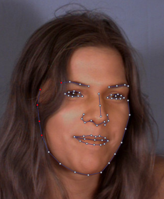
First off, here’s an example of CLMtrackr tracking a face real-time:
How does CLMtrackr work:
CLMtrackr is based on the algorithms described in this paper by Jason Saragih & Simon Lucey, more precisely “Face Alignment through Subspace Constrained Mean-Shifts”. The explanation in the paper is pretty dense, so I’ll try to do a simpler explanation here.
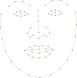
Our aim is to fit a facial model to a face in an image or video from an approximate initialization. In our case the facial model consists of 70 points, see below.
The algorithm fits the facial model by using 70 small classifiers, i.e. one classifier for each point in the model. Given an initial approximate position, the classifiers search a small region (thus the name ‘local’) around each point for a better fit, and the model is then moved incrementally in the direction giving the best fit, gradually converging on the optimal fit.
I’ll go on to describe the facial model and classifiers and how we create/train them.
Model
A face is relatively easy to model, since it doesn’t really vary that much from person to person apart from posture and expression. Such a model could be manually built, but it is far easier to learn from annotated data, in our case faces where the feature points have been marked (annotated). Since annotating faces takes a surprisingly long time, we used some existing annotation from the MUCT database (with slight modifications), plus some faces we manually annotated ourselves.
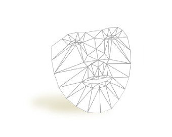
To build a model from these annotations, we use Principal Component Analysis, or PCA for short. We first calculate the mean points of all the annotations, and then use PCA to extract the variations of the faces as linear combinations of vectors, or components. Very roughly explained, PCA will extract these components in order of importance, i.e. how much of the variation in face can be accounted for by each component. Since the first handful of these components manage to cover most of the variation in face postures, we can toss away the rest without any loss in model precision.
The first components that PCA extract will usually cover basic variations from posture, such as yaw, pitch, then followed by opening and closing mouth, smile, etc.
Any facial pose can then be modelled as the mean points plus weighted combinations of these components, and the weights can be thought of as “parameters” for the facial model. Check out the complete model here
From the PCA, we also store the eigenvalues of each component, which tells us the standard deviation of the weights of each component according to the facial poses in our annotated data [1], which is very useful when we want to regularize the weights in the optimization step.
Note : PCA is not the only method you can use to extract a parametric face model. You could also use for instance Sparse PCA which will lead to “sparse” transformations. Sparse PCA doesn’t give us any significant improvements in fitting/tracking, but often gives us components which seem more natural, which is useful for adjusting the regularization of each components weights manually. Test out a parametric face model based on Sparse PCA.
[1] : this also means that it is important that the faces used for training the model is a good selection of faces in a variety of different poses and expressions, otherwise we end up with a model which is too strictly regularized and doesn’t manage to model “extreme” poses
Patches
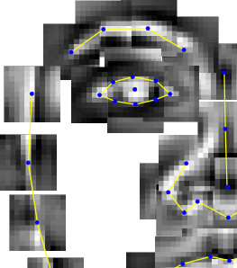
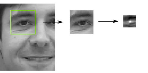
As I mentioned, we have one classifier for each each point in the model, so 70 classifiers altogether for our model. To train these classifiers, say for instance the classifier for point 27 (the left pupil), we crop a X by X patch centered on the marked position of point 27 in each of our annotated facial images. This set of patches are then used as input for training a classifier.
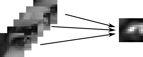
The classifier we use could be any classifier suited for image classification, such as Logistic Regression, SVM, regular Correlation Filters and even Random Forests, but in our case we implemented a SVM classifier with an linear kernel (which is what the original paper suggests), and also a MOSSE filter. More about implementation issues of these below.
When using these classifiers in fitting the model, we crop a searchwindow around each of our initial approximate positions, and apply the respective classifier to a grid of Y by Y pixels within the searchwindow. We thus get a Y * Y “response” output which maps the probability of each of these pixels being the “aligned” feature point.
Optimization
So, given that we have the responses from our classifiers, how do we apply this information to fit the facial model in the best possible way?
For each of the responses, we calculate the way the model should move in order to go to the region with highest likelihood. This is calculated by mean-shift (which is roughly equivalent to gradient descent). We then regularize this movement by constraining the “new positions” to the coordinate space spanned by the facial model. In this way we ensure that the points of the model does not move in a manner that is inconsistent with the model overall. This process is done iteratively, which means the facial model will gradually converge towards the optimal fit [2].
[2] : this happens to be a case of expectation-maximization, where finding the best movement according to responses is the expectation step and regularization to model is the maximization step
Initalization & checking
One thing that has to be noted is that since the searchwindows we use are pretty small, the model is not able to fit to a face if is outside the “reach” of these searchwindows [3]. Therefore it is critical that we initialize the model in a place not too far from it’s “true” position. To do so, we first use a face detector to find the rough bounding box of the face, and then identify the approximate positions of eyes and nose via a correlation filter. We then use procrustes analysis to roughly fit the mean facial model to the found positions of the eyes and nose, and use this as the initial placement of the model.
Altogether, this is what initialization and fitting looks like when slowed down:
While we’re tracking and fitting the face, we also need to check that the model hasn’t drifted too far away from the “true” position of the face. A way to do this, is to check once every second or so that the approximate region that the face model covers, seems to resemble a face. We do this using the same classifiers as on the patches, logistic regression, only trained on the entire face. If the face model does not seem to be on top of a face, we reinitialize the face detection.
[3] : we could of course just make the searchwindows bigger, but every pixel we widen the searchwindow increases the time to fit exponentially, so we prefer to use small windows
Performance/implementation issues
The straightforward implementation of this algorithm in javascript is pretty slow. The main bottleneck is the classifiers which are called several times for each point in the model on every iteration. Depending on the size of the searchwindow (n) and the size of the classifier patches (m), the straightforward implementation is an O(m2 * n2) operation. Using convolution via FFT we can bring it down to O(n log(n)), but this is still slower than what we want. Fortunately, the linear kernels lends itself excellently to fast computation via the GPU, which we can do via WebGL, available on most browsers these days. Of course, webGL was never meant to be used for scientifical computing, only graphical rendering, so we have to jump through some hoops to get it to work.
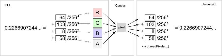
The main problem we have is that while most graphic cards support floating point calculations and we can easily import floating points to the GPU, there is no way to export floating point numbers back to javascript in WebGL. We are only able to read the pixels (which only support 8-bit ints) rendered by the GPU to the canvas. To get around this, we have to use a trick : we “pack” our 32-bit floats into four 8-bit ints, “export” them by drawing them to canvas, then read the pixels and “unpack” them back into 32-bit floats again on the javascript side. In our case we split the floats across each of the four channels (R,G,B,A), which means that each rendered pixel holds one float. Though this seems like a lot of hassle for some performance tweaks, it’s worth it, since the WebGL implementation is twice as fast as the javascript implementation.
Once we get the responses, we have to deal with the matrix math in order to do regularization. This is another bottleneck, and really exposes the huge differences in speed of numerical computing between the javascript engines of the different browsers. I used the excellent library “numeric.js” to do these calculations - it currently seems to be the fastest and most full-featured matrix library out there for javascript, and I highly recommend it to anyone thinking of doing matrix math in javascript.
In our final benchmark, we managed to run around 70 iterations of the algorithm (with default settings) per second in Chrome, which is good enough to fit and track a face in real-time.
Improvements
CLMtrackr is by no means perfect, and you may notice that it doesn’t fit postures that deviates from the mean shape all that well. This is due to the classifiers not being discriminate enough. We tried training the classifiers on the gradient of the patches, but this is slower and not all that much better overall. Optimally each response would be an ensemble of SVM, gradient and local binary filters (which I never got around to implementing), but for the current being, this would probably run too slow. If you have some ideas to fix this, let me know!
Another improvement which might improve tracking is using a 3D model instead of a 2D model. Creating a 3D model is however a more difficult task, since it involves inferring a 3D model from 2D images, and I could never get around to implementing it.
Oh, and there’s also things such as structured SVM learning, but that will have to wait until another time.
Have you used CLMtrackr for anything cool? Let me know! If you liked this article, you should follow me on twitter.